by Christian Dickel

There are different kinds of scientific papers. Some are like James Joyce’s Ulysses – you really want to read them but you have never made it through. There are the English classics – they are timeless and awe-inspiring. Like Shakespeare, some papers have changed the english language and, for example, teleported the wrong ideas into the heads of numerous journalists. In my group, we have a Harry Potter paper that we read again and again and keep discovering new insights. This is Jens Koch et al.’s 2007 classic “Charge insensitive qubit design derived from the Cooper pair box”, which introduced the transmon qubit.

In the first blog article of this series, I tried to explain conceptually how we make artificial atoms from superconducting circuits. Here, I want to get more specific and introduce cavity (and circuit) quantum electrodynamics and give my Cliff’s Notes on the transmon qubit.

Again, the blog post is rather long, but I have marked more technical sections with a *.

From cavity to circuit quantum electrodynamics

In the first blog post I mentioned spectral lines: atoms only react to light at certain frequencies that depend on the particular atom. Light-matter interaction was at the heart of quantum mechanics from the start, but atoms usually only couple weakly to light. To study more interesting physics, the interaction of atoms and light needed to be enhanced. For this reason, cavities were introduced. Basically scientists used two mirrors whose distance was a multiple of the wavelength of one of the energy transitions of the atoms to produce a standing wave of light at that frequency, as illustrated above. You can just think of a photon passing by the atom multiple times while bouncing between the mirrors and therefore interacting more strongly with the atom.

Sketch of an atom trapped in an optical cavity.

These cavity-atom systems were instrumental in studying single atoms coupled to single photons, because now a single atom could induce large enough changes in light fields to be measured. The success of these experiments inspired our experiments: cavity quantum electrodynamics with atoms and optical photons was translated to circuits and microwave photons under the name circuit quantum electrodynamics.

Circuit diagram of a transmon qubit-cavity system

We essentially try to build an electrical circuit that behaves exactly like the cavity-atom system. Our cavity is the harmonic oscillator circuit (blue) already mentioned in the previous blog post. The energy in that circuit oscillates between the capacitor and the inductor. In the quantum limit the cavity circuit can store single photons of light and couple them to our artificial atoms. The cavity-aided strong coupling has since been used to achieve fast high-fidelity readout in superconducting qubits. But the cavity by itself cannot be used as a quantum information processor. All the different states of the cavity form a ladder of increasing photon number with equal spacing. If we want to drive the system from one state to the next higher, we actually drive it all the way up the state-ladder. In fact, apart from showing quantization of light, cavities do not exhibit interesting quantum dynamics like superpositions and entanglement by themselves. For that an additional circuit element is needed.

The Josephson Junction*

So we need a circuit element in addition to the capacitor, inductor and resistor, that makes a state ladder where each step between two levels is unique: In our case this is brought about by the Josephson junction. In the previous post, I mentioned that superconductivity means that all the current-conducting electrons start forming these Cooper pairs which in turn collapse into a massive entangled ground state. As a consequence, a macroscopic island of superconductor is described by the number of Cooper pairs and by the phase of the condensate. Brian Josephson – a 22 year old PhD student at the time – wrote a paper on the problem of two weakly coupled superconducting islands which lead to our new circuit element: The Josephson junction. Naturally this only exists in superconducting circuits. Cooper pairs can “tunnel” through the junction from one island to the other. This tunneling gives rise to a current. Josephson derrived the relationship between the tunneling current \(I\), and the voltage difference and superconducting phase difference between the islands \( V\) and \( \phi\) respectively:

\(
I=I_c \sin(\phi)
\)

\(
V=\frac{\Phi_0}{2 \pi} \frac{\partial \phi}{\partial t}
\)

Here, \( I_c \) is a critical current that is a parameter of any Josephson junction and \( \Phi_0\) is the superconducting flux quantum, a natural constant. Using these Josephson relations and basic relations between current and voltage, one can come to realize that the Josephson junction can be interpreted as an inductor – inductance being the quantity that relates voltage to the time derivative of the current:

\(
V=L_J \frac{\partial I}{\partial t} \quad \rm{ with } \quad L_J = \frac{\Phi_0}{2\pi I_c \cos(\phi)}
\)

But the Josephson inductance \( L_J \) implicitly depends on the current \(I\) itself via the phase \( \phi \), which a normal inductance does not.

The transmon qubit

This is of course a simplified account but the idea to make a small change to the harmonic oscillator circuit by substituting the inductor for a Josephson junction is one way to arrive at the transmon qubit. The red circuit above made of two Josephson junctions and a capacitor in parallel will have a slight deviation from the parabolic potential of the harmonic oscillator and therefore the energy transitions of the different states will be different. We can then just shine light at the frequency \( \omega_{01}\) to transfer it from the \( \vert 0 \rangle \) state to the \( \vert 1 \rangle \) state and vice versa. If \( \omega_{12} \) and the other transition frequencies are different enough, our drive can be selective, meaning we can change the cavity state from the \( \vert 0 \rangle \) to the \( \vert 1 \rangle \) state without accidentally going into the other states. We usually only use the first two states of the superconducting circuit to encode information and only sometimes have to take into account the higher states – mostly as a place where information can get lost.

Energy landscape of the transmon circuit. Note that the vertical spacing between the energy levels is different everywhere.

It was immediately pointed out that the small difference of \( \omega_{01} \) and \( \omega_{12} \), which we call the anharmonicity, puts a time limit on the qubit operations, because if pulses are short in time it means they will become broader in frequency. If they are too short, they would also drive the transition from state \( \vert 1 \rangle \) to state \( \vert 2 \rangle \). However, theorists quickly figured out pulse schemes that reduced this problem. While having other states the information can get lost in is a limitation, currently this has not been the limiting factor for transmon qubit performance.

Later on, in coupling two transmon qubits, schemes were developed that explicitly use the higher levels. The higher levels also play a role in the transmon-cavity coupling. The almost-harmonic-oscillator qubit is a blessing and a curse, but the simplicity of the circuit and the noise resilience I will explain further below in this blog post have made the transmon one of the most succesful qubits to date.

The actual quantum hardware

This was all theory, but lets now look at actual parameters and some pictures of real chips. We have chosen parameters to get the desired transition frequencies (the formulas for getting them from the circuit capacitances and the Josephson inductance are found in Koch et al.) and use electrostatic simulations to design a chip. The chip is then fabricated in a cleanroom with technologies similar to those used in making computer chips.

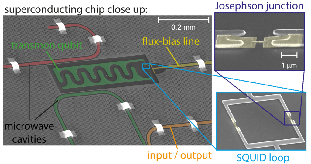
But let’s take a close look. An electron microscope allows us to see even the smallest features of our design and is an invaluable tool for diagnosing problems in the realization. Pictures are black and white but I added false colors to highlight different elements. Below, you can see the interdigitated transmon capacitor, colored in green. As you can see, the capacitor of our “atom” is about half a millimeter long. The cavity has a total length of several centimeters. The SQUID loop that I will explain later is at the end of the capacitor and connects the two islands via the Josephson junctions. The loop is 16.5 \(\mu\)m x 20.\(\mu\)m in size. The Josephson junction is a ~nm thick oxide barrier sandwiched between two aluminum layers. The bottom layer connects to the left capacitor island, the top layer to the right island. Seen from the top, the smallest feature of the the Josephson junction is about 30 nanometers wide. The two microwave cavities, here in red and green, are essentially on-chip cables that are cut of or shorted to grounds on the ends. They are several millimetres long. The green cavity is used to read out the transmon state and couples to the orange line which leads through a coaxial cable all the way up to room temperature, where the readout results are registered. The white bridges are used to connect the ground planes of the chip across the on-chip cables. So the design parameters span six orders of magnitude!

Electron microscope image of a real transmon chip.

Tuning knobs

Our qubit energies are mostly determined by the circuit parameters which cannot be changed once the circuit is made. But being able to tune the qubit energies post-fabrication can be useful. We use the previously mentioned SQUID loop, a loop of two Josephson junctions, because it behaves like one Josephson junction which can be tuned by the magnetic field that flows through the loop. SQUID is a witty acronym for Superconducting Quantum Interference Device – the interference of currents going clockwise and counter-clockwise through the loop is influenced by the magnetic field. Passing a current through the flux bias line (yellow above), the magnetic field changes and the qubits frequency will change as a function of that current. We use this tuneability of the frequency to perform fast operations and to manage chips of higher complexity where frequencies of many qubits need to be adjusted for optimum performance. This some experimental data showing a transmon’s resonance frequency responding to a current.

response diagram of energy vs. current of a transmon.

The transmon also reacts to electric fields. Atoms also show behavior like this and we actually use the atomic physics term “Stark effect” in analogy for qubit energies shifting in the presence of external fields. We use capacitive coupling to microwave lines in order to manipulate the qubit. The capacitive coupling to a cavity is used to read out the qubit state. In Koch et al., you can find the theory on how that readout works.

Qubits and noise: Charge and flux sensitivity*

On paper one can draw many different circuits, calculate Hamiltonians and chose two states to use as a qubit. Here is a review article that covers most common superconducting qubit designs – some of them have already fallen out of use. The devil is in the details. Qubits need to be in the right frequency range and their circuits need to allow for fast manipulation, coupling them to other qubits when coupling is wanted and readout with high fidelity. The trivial way to make something noise insensitive is to just completely decouple it from the environment, but that doesn’t make for practical computer hardware! The Koch et al. paper covers most of these topics but more importantly it tries to derive the effects of real-world noise and shows the transmon is viable despite of them.

When the transmon was first introduced, its resilience to charge noise, the most problematic kind of noise for most quantum devices at the time, was the main selling point. In analogy to the LC-circuit, in a transmon energy is stored in the capacitor and in the Josephson junction. If we play with these two energies, we can make transmons with different transition frequencies and different anharmonicities. The larger the capacitive energy, the stronger the transmon will couple to electric fields. So in order to be insensitive to charge noise, one has to make qubits with a small charging energy. However, this lead to a small anharmonicity. Initially people overestimated the problems that came with a low anharmonicity, so the first superconducting qubit had the same circuit but chose parameters that made it very charge sensitive. But it was noticed by Jens Koch and his collaborators, that the transmons charge sensitivity goes down exponentially with the ratio of the Josephson energy and the charging energy, while the anharmonicity only scales with a weak power law, which means it becomes much slower than the charge sensitivity. Therefore, at the point where one is basically charge insensitive, there is still enough anharmonicity left in order to have a valid qubit. All the while the transmon can still be manipulated, read out and coupled to other transmons.

In the paper, the dependence of the transmon transition frequency on the flux through the loop with two Josephson junctions is also worked out and they try to estimate the limit this noise imposes. As you can see in the measured data of flux vs frequency above, at the maximum the dependence of frequency on flux is very weak. As one moves away from the maximum, the sensitivity to flux increases. The linewidth of the transmon peak in this data also increases visibly, which makes sense, because the linewidth is related to the coherence which is reduced by increased noise sensitivity. The reason I point this out, is that the useful tuneing range of the transmon is limited. Quantum systems have to be controllable but the perfect qubit has exactly the control knobs it needs and not more.

The future of the transmon

Currently our superconducting quantum computer research in Delft is based on transmon qubits and so are the research efforts of IBM and Google (Googles Xmon is a transmon qubit with an X-shaped capacitor). The startup Rigetti Computing is exploring transmon circuits and at Yale University, where the transmon was developed, they are using the transmon circuit in order to manipulate cavity states which in their scheme become the real information carriers. At this point transmon circuits are scaling up to tens of qubits. If a chip can be made where these qubits can work together to form a large scale quantum processor, the transmon might be the transistor of the quantum computer. But there are other circuits being developed and superconducting circuits are not the only platform for quantum computing that is being considered. So the next few years will be the key years for the transmon qubit.

About Christian Dickel

Christian Dickel

Chris came to the Netherlands for the food and the weather but stayed for the quantum computer work. Apart from work he enjoys playing music with friends, ranting and soap-boxing.