If you are an experimentalist and you want to check if you have a qubit in your experiment, then you may know that a good way to that is to perform a Rabi experiment. You drive your qubit and, ideally, you see coherent oscillations that tell you that indeed you have a qubit.
What I am interested to find out: how did you learn about Rabi oscillations for the first time? I wonder this time and again, because often Rabi oscillations are only found in late chapters of quantum mechanics textbooks, if at all. I find that surprising because, for me, the basic physics of Rabi oscillations represents the simplest and the most comprehensible example of quantum mechanics we can think of.
While this maybe be subjective, I like to think that quantum mechanics is easier to understand if we start by considering a system of just two discrete states. Classically, this can correspond to one classical information bit (that can have values 0 and 1), in the quantum system this minimal example corresponds to a two-level quantum system — a qubit. For me, a system that can be 0 or 1 is much simpler to think about than a continuous function over the coordinate \(x\) defined to have finite L2-norm.
The wave-function of such two-level quantum systems lives in a complex two-dimensional Hilbert space and is described by the vector \(\left| \psi \right\rangle = \begin{bmatrix} \alpha \\ \beta \\ \end{bmatrix}.\) Following the rules of quantum mechanics, we need to impose \(\left| \alpha \right|^{2} + \left| \beta \right|^{2} = 1\) because \(\left| \alpha \right|^{2}\) and \(\left| \beta \right|^{2}\) are the probabilities to find the two basis states if you were to measure system in a real experiment. Now our wavefunction is fully described and we did not have to integrate anything. I think that is very elegant.
Next up, we consider a general Hamiltonian for the two-level quantum system. For simplicity, we will consider the Hamiltonian to be real; any real Hamiltonian of a qubit system can be written in the following form: \(H = \begin{bmatrix} \Delta_{1} & \Omega \\ \Omega & \Delta_{2} \\ \end{bmatrix}.\) Here the requirement that the Hamiltonian is Hermitian sets the off-diagonal elements to be equal. For the interested reader let me mention that we often refer to \(\Delta_{1}\) and \(\Delta_{2}\) as the self-energies of the basis states while \(\Omega\) is the coupling energy between the two. This Hamiltonian is quite simple and the Schrodinger equation \(H\left| \psi \right\rangle = E|\psi\rangle\) can be solved fully analytically (I leave that as an exercise for the motivated reader — or Wolfram Alpha).
To simplify the problem just a bit more, we consider the case of \(\Delta_{1} = \Delta_{2} = 0\). Here we find the eigenvalues \(E_{\pm} = \pm \Omega\) with the eigenvectors \(\left| \psi_{\pm} \right\rangle = \frac{1}{\sqrt{2}}\begin{bmatrix} 1 \\ \pm 1 \\ \end{bmatrix}.\)
The final basic concept of quantum mechanics that we need is that of time evolution. In quantum mechanics, during time evolution any eigenstate with energy \(E\) gets a pre-factor of \(e^{- iEt/\hbar}\). So, if we start in the state \(\left| \psi_{0} \right\rangle = \begin{bmatrix} 1 \\ 0 \\ \end{bmatrix} = \frac{1}{\sqrt{2}}(\left| \psi_{+} \right\rangle + \left| \psi_{-} \right\rangle)\), then the state at time \(t\) is found to be \(\left| \psi\left( t \right) \right\rangle = \frac{1}{\sqrt{2}}\left( e^{- \frac{i\Omega t}{\hbar}}\left| \psi_{+} \right\rangle + e^{\frac{i\Omega t}{\hbar}}\left| \psi_{-} \right\rangle \right).\)
The question that I have is now: what is the probability that we are in the state \(\left| \psi_{1} \right\rangle = \begin{bmatrix} 0 \\ 1 \\ \end{bmatrix}\) at any given time? With just a bit of trigonometry, we find \(P_{\left| 1 \right\rangle}(t) = \sin\left( \frac{\Omega t}{\hbar} \right)^{2}.\) This formula tells you that the probability for the system to be in the state \(\left| \psi_{1} \right\rangle\) oscillates with the frequency \(\Omega/\hbar\ \)– the Rabi frequency!
With this very small exercise, I hope to have convinced you that Rabi oscillations are simple to derive and instructive to think about. It is also very easy to see what happens when \(\Delta_{1}\) and \(\Delta_{2}\) are different from zero with just a bit of extra calculations. To conclude, I think the Rabi oscillation is arguably the simplest example in quantum mechanics and should be taught as such. The Rabi oscillation is, in that sense, a concept that can bridge the gap between the frontiers of quantum research and students just starting their journey into the quantum world. Moreover, if you are doing research that involves qubits, knowing how to derive Rabi oscillations with various tweaks to the Hamiltonian will become useful in your everyday work in the lab, I promise 😉
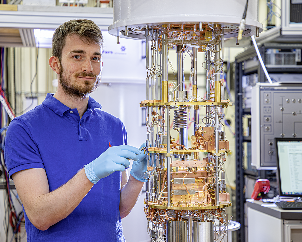
Christian Kraglund Andersen joined QuTech as an assistant professor in March 2021. He obtained his PhD in 2016 from Aarhus University in Denmark. During his PhD, he was also a visiting student of University of Sherbrooke in Canada for two short periods of time. After his PhD, Christian joined ETH Zurich in Switzerland to work in lab of Prof. Andreas Wallraff on large-scale superconducting quantum devices. Christian’s current research at QuTech is focused on developing the next generation of high-quality superconducting qubits.


 Christian Kraglund Andersen joined QuTech as an assistant professor in March 2021. He obtained his PhD in 2016 from Aarhus University in Denmark. During his PhD, he was also a visiting student of University of Sherbrooke in Canada for two short periods of time. After his PhD, Christian joined ETH Zurich in Switzerland to work in lab of Prof. Andreas Wallraff on large-scale superconducting quantum devices. Christian’s current research at QuTech is focused on developing the next generation of high-quality superconducting qubits.